Bagging and Random Forests: Reducing Bias and variance using Randomness
This article will provide an overview of the famous ensemble method bagging and even cover the topic of random forests.
Brief topics that we will cover are :
- Introduction to Ensemble Learning
- Bagging and its pseudo code
- Conditions to use Bagging
- Pros and Cons of Bagging
- Random forest and its pseudo code
- Hyperparameters in Random forests
- Real-life examples
- Building Bagged trees and Random forest classifier using scikit learn
So let’s get started!
Ensemble Learning:
Ensemble learning is a great way of improving the performance of your model. From the name itself, it is evident that we use a collection (or ensemble) of different models or base learners and then combine their predictions to generate a better final prediction.
Ensemble learning is useful for improving the predictions of weak learners, by combining their predictions. Not only is the accuracy of predictions increased (predictions are closer to the true value), but the spread of predictions also goes down. This means that the best and worst-case values are closer to the mean prediction. Ensemble learning can be specifically useful in striking the right balance between bias and variance.
Bagging and boosting are the most common methods of ensemble learning. While bagging takes place parallelly, boosting is a sequential process.
What is Bagging?
Bagging (also known as bootstrap aggregating) is an ensemble learning method that is used to reduce variance on a noisy dataset.
Imagine you want to find the most selected profession in the world. To represent the population, you pick a sample of 10000 people. Now imagine this sample is placed in a bag. You take 5000 people out of the bag each time and feed the input to your machine learning model. And then you place the samples back into your bag. Once the results are predicted, you then use the maximum voting to pick the best results. This is nothing but the basis of bagging. Now let's go over it in a more detailed way.
It is a process that involves training similar models by creating different samples from the given training data. First, diverse samples of data are randomly generated from the training data. It is important to note here that the samples are selected with replacement — which is to say that the same individual data points can be selected more than once.
After this, the weak or base learners are trained independently on these samples (called bootstrap samples). The entire process of learning takes place parallelly.
The third step involves combining the predictions with the individual models. This aggregation is done in several ways, one of which is by taking an average of all the individual predictions. The final prediction is thus better- more accurate, robust, and with less spread of predictions.
In generalized bagging, this final prediction is made by combining the predictions of different models which were trained on different samples.
This image depicts the basic three steps involved in bagging
Pseudocode for Bagging:
WHEN CAN WE USE BAGGING?
Bagging efficiently decreases the variance of an individual base learner (i.e., averaging reduces variance); but, bagging does not necessarily improve upon an individual base learner due to the aggregation process. Some models have more variance than others.
Bagging is extremely effective for learners with unstable, high variance bases.
Now, what are unstable classifiers?
These are bases that tend to overfit i.e these are classifiers that have a high variance. Two examples of such types of classifiers are unpruned decision trees and k-Nearest neighbors with a small k value.
However, it is seen that bagging offers very little to no improvement for algorithms that are more stable i.e algorithms that have a high base value. The graph below shows the bagging of 100 base learners :
High variance models such as C) Decision trees benefit most from bagging compared to low variance models like A) Polynomial regression which shows almost no improvement
ADVANTAGES OF USING BAGGING
i)The primary benefit of bagging is that it allows numerous weak learners to work together more effectively than a single good learner.
ii)It aids in the reduction of variance, as well as the avoidance of overfitting.
iii)It ensures consistency and improves the accuracy of machine learning algorithms used in statistical classification and regression.
iv)We select data through resampling with replacement, hence there are repetitions/duplicate values. The samples which have not been used in any sample dataset are called out of bag (OOB). This can be used for validation.
DISADVANTAGES OF BAGGING
i)It becomes computationally expensive since we must utilize numerous models, and it may not be acceptable in certain use scenarios.
ii)If it is not adequately modeled, it may result in high bias and therefore underfitting.
Concept of Parallelization
Bagging can be quite expensive computationally but as it involves training models which are completely independent we can use parallelization.
We can separate models parallelly and later average out their prediction values. This makes bagging quite easier compared to boosting (the other ensemble method).
RANDOM FORESTS
We will now explore the algorithm of random forests which builds upon the theory we learned in bagging. Let’s look into a real-life analogy of random forests.
Rahul wants to take his girlfriend out for a date on valentine’s day but he isn’t sure about which place to take her to. So he asks the people who know her best for suggestions. The first friend he seeks out asks him about her past travels. Based on the answers, he will give Rahul some advice.
Then Rahul starts asking more and more of his friends to advise him and they again ask him different questions they can use to derive some recommendations from. Finally, Rahul chooses the places that were recommended the most to him, which is the typical random forest algorithm approach.
Random forest is an extension of bagging that also randomly selects subsets of features used in each data sample. We do so to avoid correlation among the trees.
Suppose there was a strong predictor in the dataset along with other moderately strong predictors. If we would make bagged trees then most of the trees would use the strong predictor for the split and hence most or all trees would be correlated. Correlated predictors cannot help in improving the accuracy of prediction.
By taking a random subset of features, Random Forests systematically avoids correlation and improves the model’s performance.
Below shows a simple Random forest classifier that uses 3 decision trees :
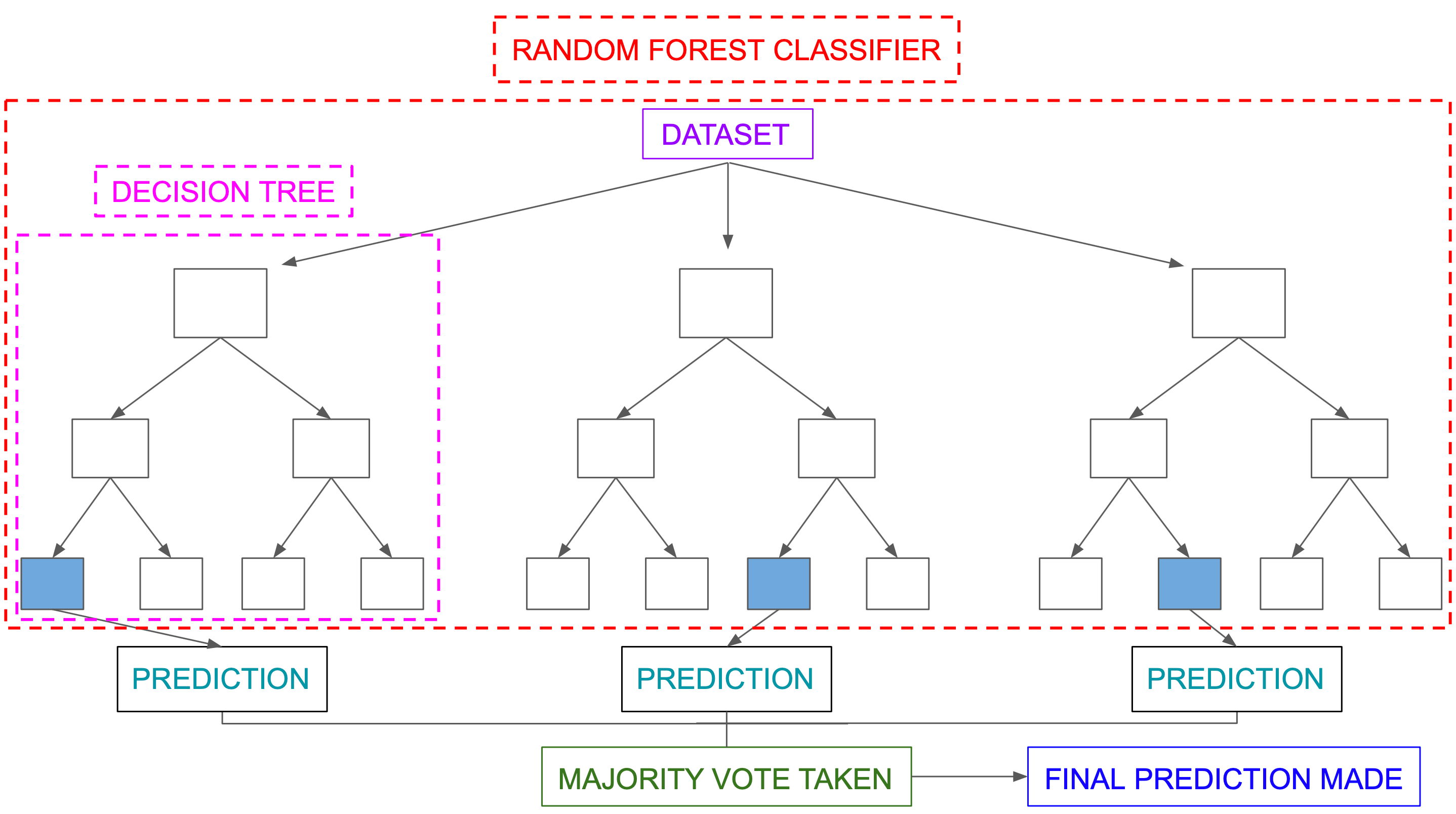
Random forests perform split-variable randomization where each time a split is to be performed, the search for the split variable is limited to a random subset of ‘m’ features among the total ‘p’ features. Below is its pseudo-code :
HYPERPARAMETERS IN RANDOM FORESTS
Now let’s dive into some of the hyperparameters involved in random forests :
i) Number of trees
The number of trees needs to be large enough to stabilize the error. A general rule of thumb is to start with ( p x 10) trees and then adjust accordingly.
More trees provide robust and stable error estimates but the computational expenses also increase linearly.
This image shows how the error varies with the number of trees for the Ames dataset. Ames dataset has 80 features and starting with 80 x 10 gives good results.
ii) Number of features to consider at any given split
Let ‘m’ be the hyperparameter that controls the split variable randomization feature. This is the number of random features selected out of the total ‘p’ features.
When there are few relevant predictors then a higher value of m works well as it ensures the selection of a stronger predictor. When there are too many strong predictors then a lower value of m is preferred. Generally m = p/3 for regression and m = √p for classification tasks.
This image shows how error varies with m for the Ames Housing dataset. We can see m=21 performs the best for this data.
iii) Tree Complexity
Random forests are built on individual decision trees. Hence tree complexity also involves various hyperparameters such as the number of terminal nodes, max depth.
This affects the run time more than the error estimate. This can be seen from the graphs below :
Real-Life Examples
i) Healthcare: Bagging has been used to form medical data predictions. Ensemble methods are used for gene and/or protein selection to identify a specific trait of interest. Random forests are used for various purposes in the healthcare domain like disease prediction using the patient’s medical history.
ii) Banking Industry: Bagging and Random Forests can be used for classification and regression tasks like loan default risk, credit card fault detection.
iii)IT and E-commerce sectors: Bagging can also improve the precision and accuracy in IT systems, such as network intrusion detection systems. Random forests can be used for product recommendation, price optimization, etc.
Let’s Code a bit!
Importing Libraries
Loading the dataset and normalizing
Splitting the dataset
Training a decision tree on the normalized dataset
Training a bagged tree
Training a Random Forest
I hope this article would have given you a solid understanding of this topic. If you have any suggestions or questions, do share in the comment section below.
So, revise, code, and watch out for our next article!
Follow us on:
Thanks for reading! ❤